Blog

Statistics extension for TMS Analytics & Physics developing library

Friday, May 18, 2018

TMS Analytics & Physics developing library includes many extensions for various mathematical applications: complex numbers, linear algebra, special functions, common fractions, numerical methods. New version 2.4 introduces package for statistical analysis. The extension allows evaluating base statistical properties of real data samples (mean value, median and others), generating sequences of special numbers (Fibonacci, prime numbers and many others), creating arithmetic, geometric and harmonic progressions, working with probability distributions.

It should be noted here, that as the Analytics library allows symbolic evaluations of very complicated formulae, some statistical problems can be solved without using the special package. For an example, the Linear Algebra package includes functionality for processing array and matrix data. So, we can solve, for an example, the following problem: find the sum of ‘A’ array elements those are greater than ‘x’. The result can be calculated with the following code:



The output for the code is the following:



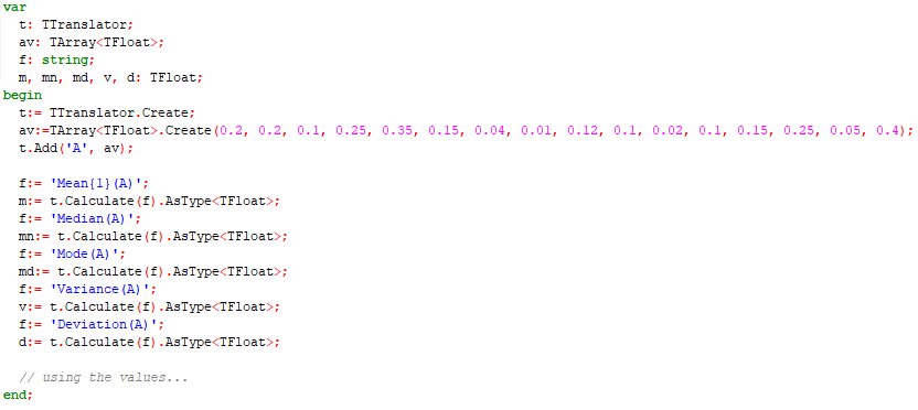
The problem is solved with the ‘if’ function that compares all items of the ‘A’ array with ‘x’ value and generates new array which contains elements of ‘A’ if the condition satisfied and 0 value if not. When the sum of the result array calculated we get the solution of stated problem. The goals of new Statistics package is providing the simplest formula for evaluating base statistical characteristics and solving statistical problems that cannot be solved without specialized library. First, let us consider evaluation of base statistical characteristics of some discrete sample values, stored in ‘A’ array. This can be done with the following code:



For this data, we get the following statistical values:

Mean of A = 0.155625
Median of A = 0.135
Mode of A = 0.1
Variance of A = 0.012124609375
Deviation of A = 0.440447215906742

As can be seen from the code above, every value calculated with one function call. The function ‘Mean{P}(A)’ here evaluates the mean value of the data. This function is parametric and the ‘P’ parameter specifies the ‘power’ of the mean (https://en.wikipedia.org/wiki/Mean#Power_mean). The parameter value can be one of the four: ‘-1’ – harmonic mean, ‘0’ – geometric mean, ‘1’ – arithmetic mean, ‘2’ – quadratic mean. In our case P=1 and we calculated the arithmetic mean of ‘A’. One of the advantages of using the symbolic capabilities of the Analytics library is that, even if some feature is not realized in the package directly, one can use the formula for this feature. Let us consider how to do this for other types of ‘mean’ values. There is so called generalized mean (https://en.wikipedia.org/wiki/Mean#Generalized_means) that is defined by the formula:



where f is a function and f-1 is its inverse. For an example, if f is exponent, then f-1 is natural logarithm. The ‘exponential’ mean function is not provided with the statistical package, but it can be easily evaluated with the following simple formula:



which produces the output:

Exponent Mean of A = 0.161840327746035

The value of ‘exponent’ mean is slightly differs from common arithmetic mean that follows from the different meaning of the characteristics.

One of main features of Statistics package is that it allows working with probability distributions and solve real statistical problems (https://en.wikipedia.org/wiki/Probability_density_function). The version supports 6 distributions: Gauss (normal), Laplace, Cauchy, Gumbel, logistic and exponential. Let us consider the following statistical problem: there is a known probability distribution for lifetime of a bacteria species. Let us suppose the distribution is Gaussian function with parameters µ and s (https://en.wikipedia.org/wiki/Normal_distribution). We need to calculate the probability that the bacteria dies on the time interval [t1..t2].
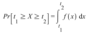
This probability defined by the formula:



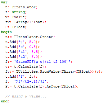
where f(x) is the probability density function (PDF) of the distribution. The value of the probability can be evaluated with the following code:



First, we added the variables for the distribution’s parameters to the translator and variables for the time interval. The function 'GaussPDF{µ s}(t1 t2 100)' produced the array of 100 values for the Gaussian PDF with specified parameters (µ=5 hours, s=0.5 hours) on the specified interval of [5.5..6.0] hours. Then we used numerical integration of the values, replacing the integral with the appropriate summation. The answer for our question is - the probability that the bacteria dies on the interval 5.5-6 hours is about 13.6%. The version 2.4 is already available. Source code of the example application for statistics analysis can be downloaded from here.

Bruno Fierens

This blog post has not received any comments yet.