Blog
All Blog Posts | Next Post | Previous Post

 TMS Analytics for nonlinear multiparametric approximation of surface data
Thursday, October 5, 2017
The new version 2.2 of TMS Analytics and Physics pack contains the nonlinear least squares approximation tools. The nonlinear approximation tasks are widely used in statistics to fit experimental data with some random distribution function.Let us consider the example of surface data fitting with the 2D Gaussian function. The Gaussian distribution of 2 variables x and y (https://en.wikipedia.org/wiki/Gaussian_function) has the following math expression:

Except the amplitude A, the distribution nonlinearly depends on four parameters: center coordinates x0, y0 and deviations sx, sy. The task of fitting data with the Gaussian function is to find optimal values of the four parameters, those minimize the error of the distribution and the experimental data zi(xi,yi), i=1..N.
The approximation task can be solved by the numerical tool with the following code:
var variables, coefficients: TArray; f: string; basis: TNonlinearBasis; cValues: TArray ; appr: TNonlinearApproximator; opt: TSolverOptions; eValues: TArray ; eValue: TFloat; begin variables:= TArray .Create('x', 'y'); // 1 coefficients:= TArray .Create('x0', 'Sx', 'y0', 'Sy'); // 2 f:= 'e^-((x-x0)^2/(2*Sx^2)+(y-y0)^2/(2*Sy^2))'; // 3 basis:= TNonlinearScalarBasis.Create(variables, coefficients, nil, f); // 4 appr:= TGaussNewtonLeastSquares.Create; // 5 appr.C0:= TArray .Create(0.1, 0.1, 0.1, 0.1); // 6 opt:= TSolverOptions.Create(true); opt.MaxIterationCount:= 100; opt.Precision:= 0.2; appr.Options:= opt; // 7 cValues:= appr.Approximate(basis, xyData, zData); // 8 // use basis with optimal coefficients end;
Line 1: Create array of variable names.
Line 2: Create array of four distribution coefficient names.
Line 3: Set up the approximation function expression.
Line 4: Create the nonlinear basis instance with specified data.
Line 5: Create the appropriate nonlinear approximator instance.
Line 6: Set up initial guess of coefficient values for nonlinear solution.
Line 7: Set up appropriate nonlinear solution options.
Line 8: Solve the problem (finding optimal values).
When optimal values of the Gauss distribution parameters found, they can be used with the basis instance to calculate the distribution function in any specified point (x,y) or for other analysis methods, like derivative calculations and so on.
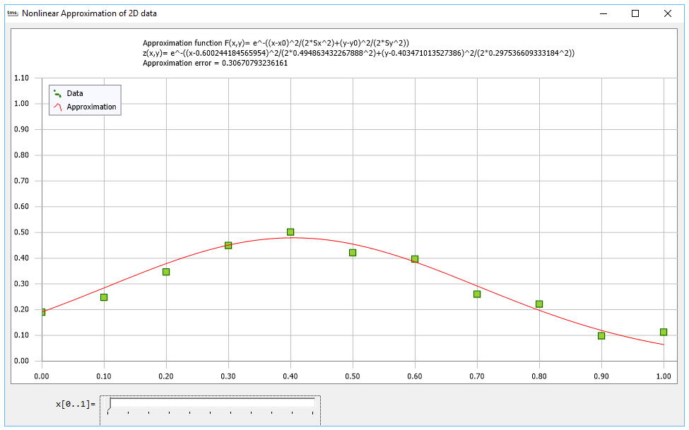
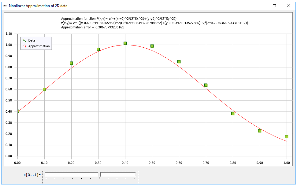
On the pictures below there are results of the approximation made with some generated noisy data. The result presented as 1D section of the 2D function for two different x values: x=0.0 and x=0.6.


In this sample, we used the TMS FNC Chart to display the values and the approximated function. The advantage of using the TMS FNC Chart is that it can be used both for VCL and FMX applications and we can use the same code to create a VCL Windows application or a FireMonkey cross platform application.
The source code of the example application can be downloaded here.
The TMS Analytics and Physics pack version 2.2 includes also many other useful numerical tools: linear least squares approximation, 1D and 2D integration, ordinary differential equation solution, function analysis. Due to the addition of array and matrix support in version 2.2, many numerical calculations can be implemented in vector form with small and compact formulae. The version can be downloaded from the product page.
Bruno Fierens

This blog post has not received any comments yet.
All Blog Posts | Next Post | Previous Post