Blog

All Blog Posts | Next Post | Previous Post

Function approximation with TMS Analytics and Physics numerical tools

Monday, June 19, 2017

The problem of data approximation (curve fitting, surface fitting) arises from many areas: economics, physics, informatics and many others. There are many libraries, realizing numerical tools for using the approximation in software applications. The TMS Analytics and Physics pack contains the approximation numerical tool which has one unique feature – it is totally integrated with symbolic calculus. Using symbolic expressions with the numerical approximation gives the developer many advantages.

Let us consider a simple case of using the approximation tool for curve fitting (one-dimensional approximation). For this case we have a set of points Pi=(xi,yi), i=1..N. From the programming point of view we just have two arrays of real values, say X and Y. The approximation problem is to build a function y=f(x) which is close to the set of points. The most popular approach of the approximation is the linear least squares (https://en.wikipedia.org/wiki/Linear_least_squares_(mathematics)). With TMS approximation tool the problem can be solved in five lines of code:

var
  approximator: TLinearApproximator;
  basis: TLinearBasis;
  variables: TArray;
  functions: TArray;
  cValues: TArray;
begin
  variables:= TArray.Create('x'); // 1
  functions:= TArray.Create('e^x', 'sin(x)', 'e^-x', 'x^2', '3^x',   'sinh(2*x)'); // 2
  basis:= TLinearScalarBasis.Create(variables, 'C', nil, functions); // 3
  approximator:= TLinearLeastSquares.Create; // 4
  cValues:= approximator.Approximate(basis, X, Y); // 5
  
  // Using the basis with optimal coefficient values.
end;

Line 1: Create the array of variable names, as this is 1D approximation, there is one variable name ‘x’ in the array.
Line 2: Create the array of approximation functions (basis functions). The functions only depend on the ‘x’ variable. The type and the number of the basis functions can be arbitrary.
Line 3: Create the basis instance with the specified arguments. The ‘C’ argument specifies the name of approximation coefficients. The ‘nil’ argument tells that there is no parameters in the functions.
Line 4: Create the appropriate approximator instance. For the linear least squares approximation it is ‘TLinearLeastSquares’;
Line 5: Calculate the approximation coefficients for the specified basis and arrays of points ‘X’ and ‘Y’.

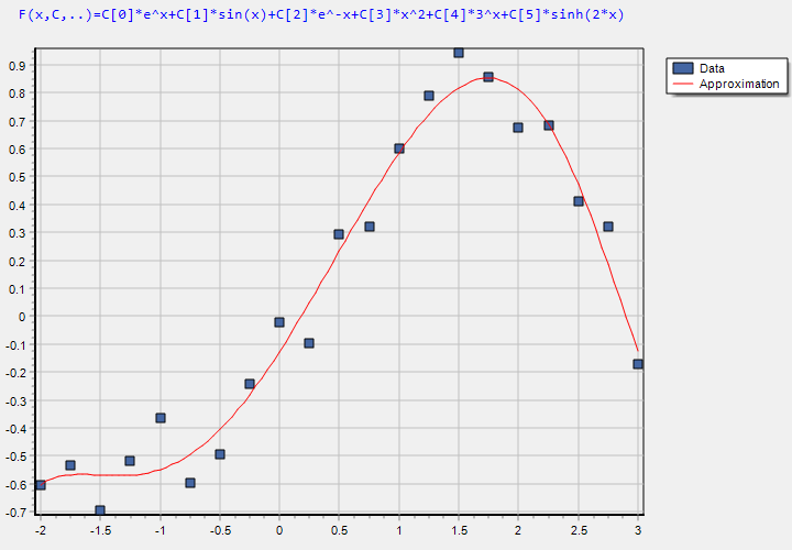
After the optimal coefficients found, we can evaluate the basis in any point and make other analytical manipulations. As example, here is the plotted approximation function with the original data points on the picture.

The main feature of the TMS numerical tools is they are totally integrated with the symbolic calculus. It brings the following advantages to the developer:
- Minimal code writing, because there is no need to write special classes for the function method references (delegates) as in other numerical libraries.
- Convenient data representation for the developer and user as math expressions, not as programming code.
- Easily using the user input data (string data) for manipulations in programming code.
- Almost unlimited choice of math expressions for manipulations, including special functions.
- Easily transfer input data and the output results via network as strings, easily storing and serializing the data.

The result of the approximation can be easily used with other numerical tools. For example, we can analyze the approximation function for the roots and special points – extremums. The code for the analysis is the following:

var
  f: string;
  sf1D: TSymbolicFunction1D;
  opt: TSolverOptions;
  points: TArray;
begin
  f:= basis.Evaluate(cValues); // 1 
  sf1D:= TSymbolicFunction1D.Create('x', f); // 2 
  opt:= TSolverOptions.Create(true);  // 3
  points:= TFunctionAnalyser.Analyse(sf1D, TNewton, opt, -2, 3, 10); // 4 
  
  // Using the points array.
end;

Line 1: Make the function expression with optimal coefficient values.
Line 2: Create the symbolic function instance for the analysis.
Line 3: Create default options for the nonlinear solver (which used for the function analysis).
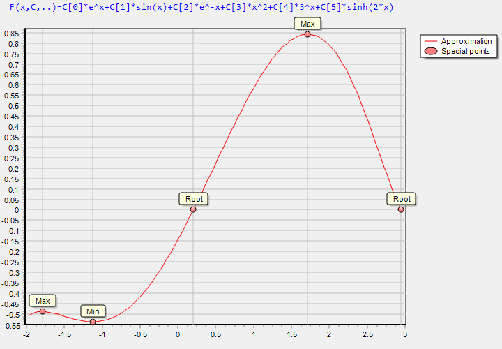
Line 4: Finding all function's special points on the interval [-2..3]. The Newton’s method used for finding roots and extremums of the function which specified with the second argument.

The result of the analysis – function’s roots and extremums, presented on the picture below.

The TMS Analytics and Physics pack includes the library with 5 ready-to-use numerical tools totally integrated with analytical features, such as symbolic derivatives. The version can be downloaded from the product page. There is the source code example for all numerical tools with the new version download.

Bruno Fierens

This blog post has received 2 comments.

1. Wednesday, July 19, 2017 at 3:32:16 PM

Is the source code of this demo available?

Holger Flick

2. Wednesday, July 19, 2017 at 3:33:43 PM

Found it... it is included with the library as Numerics.VCL